Overview
Economics are a primary concern in a well-designed strategy to reduce carbon. The potential ways to reduce carbon emissions vary dramatically on an economic basis. Some are so beneficial that they return more money to the economy than they cost, like LED lighting which is now commonplace in homes and businesses. At the other extreme are very costly solutions, although some achieve sufficient justification based on co-benefits. The amount of carbon abatement that a given method can accomplish also has limits in scale.
In this article we present a useful way to visualize this range of possibilities, which we have applied to Washington state. The data presented is a starting point for the Low Carbon Prosperity Carbon Reduction System project, with Version 0 developed from preliminary data and indicating that about 30% of our emissions through 2035 can be reduced for negative or near-zero cost.
Research during the course of the project will improve the accuracy of these assessments and provide the basis for confident investment decisions. The project is also likely to discover new opportunities in the process, especially through extensive participation across our economy, e.g. industry, solution providers, and academic colleagues.
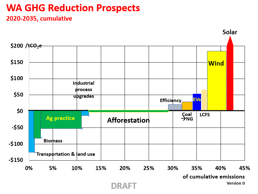
Intro to MAC Curves
A Marginal Abatement Cost Curve (MAC curve or MACC) is a succinct and straightforward method for presenting carbon emissions abatement options relative to a baseline (typically a business-as-usual pathway). A MAC curve creates an easy to understand visualization of various mitigation options or measures organized by a single metric: economic cost of emissions abatement.
MAC curves are broken into discrete “blocks.” Each block represents an individual or set of similar carbon abatement measures. For each measure, the width estimates the quantity of potential carbon emissions abatement (metric tCO2 or million metric tCO2, MtCO2) while the height estimates the marginal cost of the carbon emissions abatement ($/tCO2). This allows measures from various sectors (e.g. transportation and power) to be compared on equivalent terms, serving as an initial scoping of where abatement opportunities are potentially the largest and most cost effective. MAC curves can be powerful tools for robust initial framing and the identification of options worth further evaluating.
Some items are shown as negative cost. These are ones that return more money to the system than they cost. In a perfect market, consumers would realize this favorable payback and make the investment. The real market often can utilize modest investments, such as promotions of LEDs, to provide a stimulus to take action and overcome barriers to deployment
The first carbon-focused MAC curves date to the early 1990s, while similar curves for energy savings and other air pollutants appeared in the early 1980s (Kesicki and Ekins). To date, a Washington state specific MAC curve has not been developed, although there are examples at the national level and other states that can provide some insight. A few years ago, Oregon funded a MAC curve project carried out by the Center for Climate Strategies on an accelerated 3-month time frame, making it more of a ‘meta-analysis’ than a comprehensive modeling effort. In part due to the short study time-frame and a common problem with MAC curve studies, the Oregon study gave overlapping reduction potential between measures only cursory treatment, identifying overlapping sources of emissions reductions as a key issue.
If viewed as a useful springboard for more rigorous consideration of the various mitigation measures, MAC curves are an important policy tool. Despite the appealing simplicity of a MAC curve, useful interpretation requires a great deal of care and expertise. Simply put, MAC curves alone are “not sufficient to base policy decisions on” (ERC Netherlands). Limitations of MAC curves highlighted in literature include:
MAC CURVE LIMITATIONS
- Doesn’t capture non-market barriers to implementation;
- Offers very limited treatment of uncertainties, including “additionality” or “permanence” of abatement measures;
- Typically a snapshot that doesn’t treat the varying costs over time;
- Can mask variation from the low cost side of a measure “block” to the high cost side;
- Has difficulty accounting for interactions between different measures, and;
- Does not address other dimensions than cost (e.g. strategic, operational, or political).
In order for a MAC curve to be as robust and insightful for policy work possible, care should be taken in the approach and interpretation of MAC curves. Kesicki and Ekins offer several recommendations for the use of MAC curves:
ADVICE FOR USING MAC CURVES
- Embrace complexity;
- Pay attention to the underlying assumptions;
- Always look beyond the estimated technology costs for “unintended or perverse consequences”, and;
- Understand path dependencies.
If these caveats are given appropriate consideration, there is no doubt that a Washington-specific MAC curve could provide a great boost in identifying and teaching cost-effective strategies for deep statewide decarbonization.
For more, refer to the WaBA article Understanding Carbon Reduction: Marginal Abatement Cost Curves
Building A Washington Specific MAC Curve
To date, there is no Washington Specific MAC Curve that provides more than a cursory glance at carbon reduction measures specific to our state. The Clean & Prosperous Institute (CaPI) has decided that the time has come to undertake a more comprehensive, statewide look at MAC opportunities in our state. To that end, CaPI has launched a project to develop a MAC Curve specific to Washington that is detailed and accurate enough to be operational. This framework will allow specific project plans to be developed and launched with confidence, typically with private – public partnerships. CaPI is actively looking for partners and funders to carry this project through to a robust tool for policymakers and businesses.
There have been some pilot efforts, and discussion of additional efforts, about developing MAC curves for the state, such as: a 2013 report for CLEW by Leidos estimating $/tCO2e for a subset of transport, energy conservation, and renewables options, some discussion in the 2014 CERT Report, and the inclusion of a Pilot Cost Effectiveness Study as part of the 2015 King County Strategic Climate Action Plan. At an institutional level, the UW Climate Action Plan includes a MAC Curve of its own that also includes a dimensional analysis of barriers to implementation.
CaPI has spent several months analyzing existing literature across solutions in multiple sectors: Transportation, Power Generation, Residential/Industrial/Commercial (RCI) fuel-switching, and Agriculture/Forestry/Waste. These sectors include both carbon sequestration and avoided emission abatement options, although the two are not perfectly interchangeable and thus might be better treated separately.
Here we present preliminary findings, both in aggregate and split by sector encompassing 41 different measures (see Appendix A for a description of measures). Attempts have been made to account for and eliminate overlapping sources of carbon abatement in this preliminary assessment, most notably within the power generation sector. Our preliminary findings indicate that statewide targets can be met and exceeded without large overall costs. However more rigorous consideration of uncertainties and methodology, including consistent baseline treatment as a starting point for comparison, are needed.
Preliminary findings include:
- Potential — Of a projected 1,450 MtCO2 or equivalent cumulative greenhouse gases (MtCO2e) from 2020-2035 (Carbon Tax Assessment Model), preliminary analysis indicates the possibility to abate over 40% at an average cost of $29 / tCO2e (Figures 1 & 2). By comparison, a linear emissions reduction path to legislated targets (66.3 MtCO2e in 2035) would be an 11% cumulative reduction, while the Department of Ecology recommended limit for 2035 would be a 19% cumulative reduction;
- About 40% appears technically possible at an average net cost of zero.
- Even excluding sequestration measures, an 18% cumulative reduction from 2020-2035 at a average marginal cost of under $100/tCO2e appears achievable (Figure 3).
- Role of sequestration — Over 20% of the potential to reduce net emissions is in the form of expanded sequestration of carbon dioxide through forestry and agriculture. Adding new forests (“afforestation”) on lands with marginal economic value shows the largest potential of any measure.
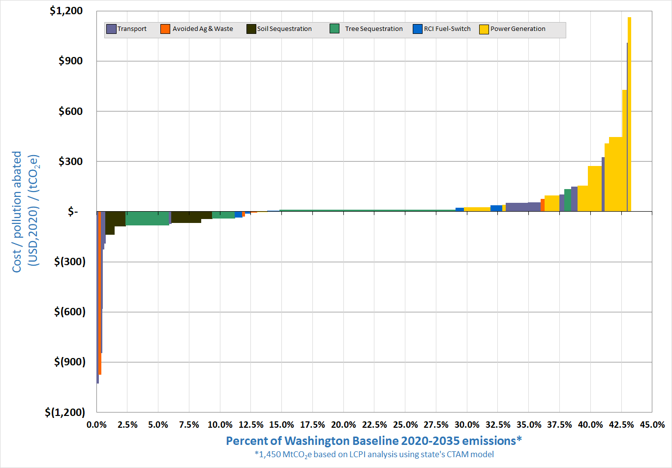
Figure 1 – Marginal Abatement Cost (MAC) Curve for all sectors evaluated in this analysis. Cumulative potential impacts, 2020-2035.
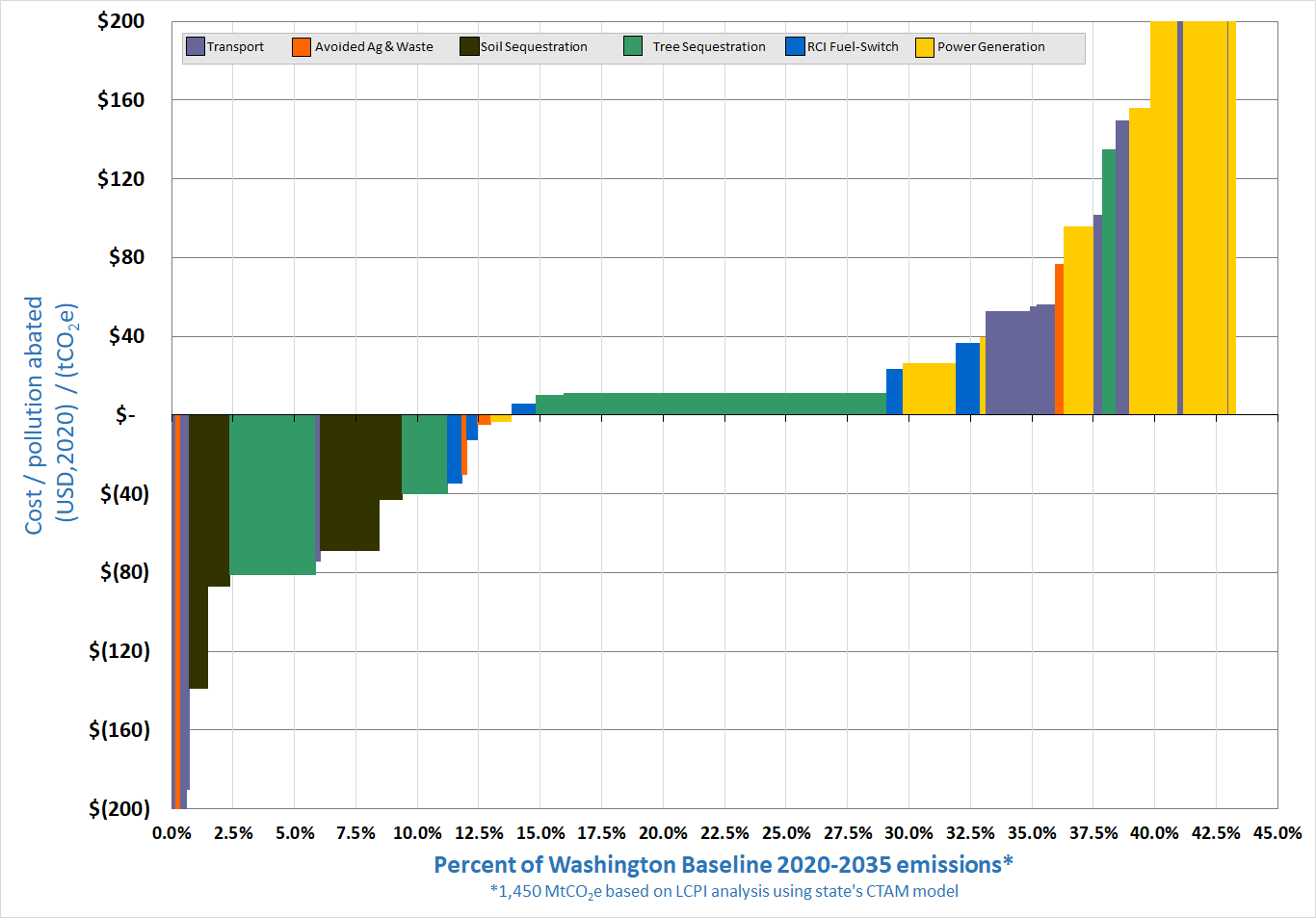
Figure 2 – MAC Curve for all sectors, cost-axis magnified. Cumulative potential impacts, 2020-2035.
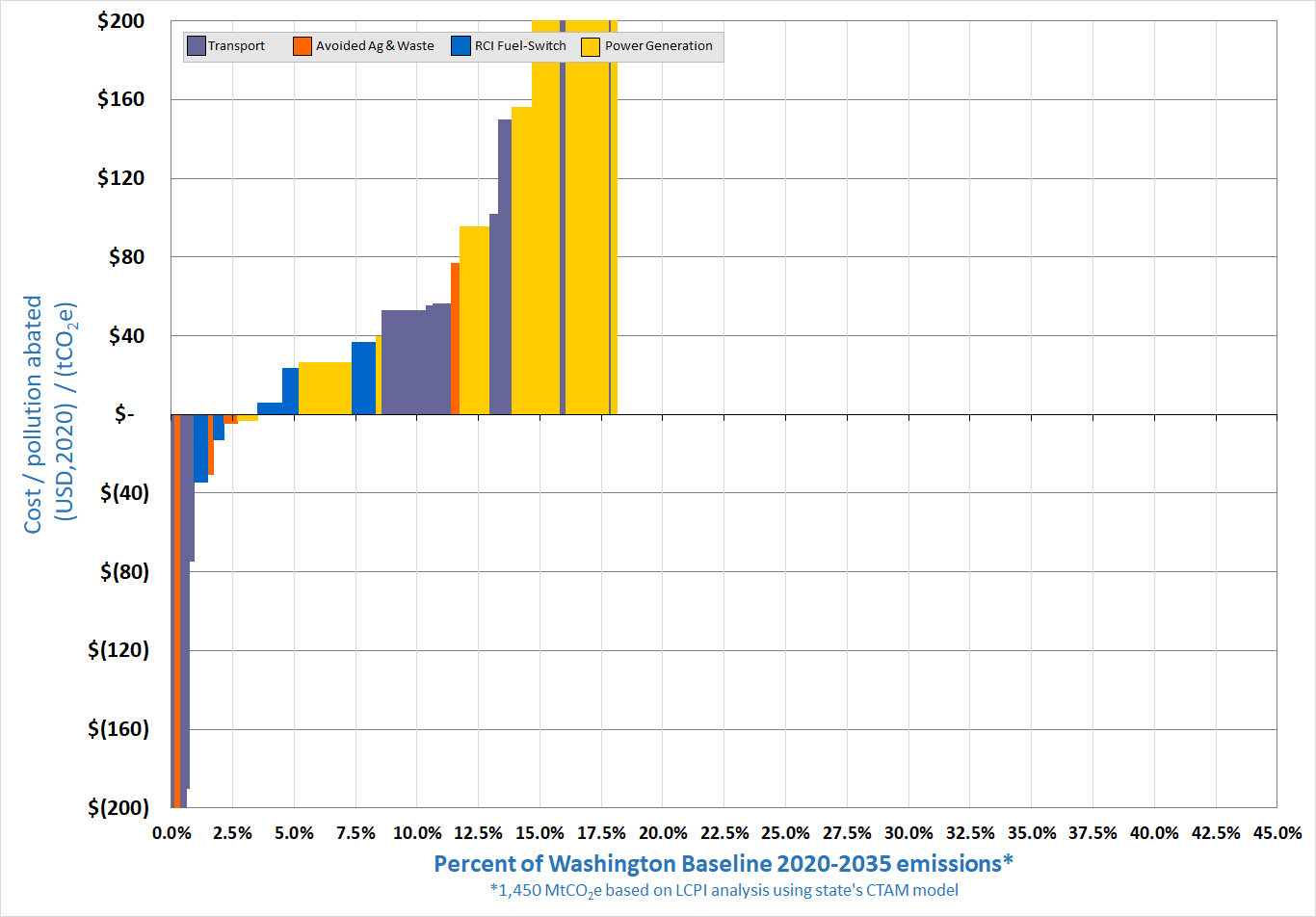
Figure 3 – MAC Curve with no sequestration, cost-axis magnified. Cumulative potential impacts, 2020-2035.
MAC Curve using aggregated categories
In practice, each of these categories of emission reductions has its own detail, with some projects costing less than others, some having more capacity potential than others, and some providing both low cost and high capacity. To give a little better perspective these can be aggregated into summary levels with averaged performance. This is displayed in Figure 4. Negative or low cost items tend to biological in nature.
Items marked by an asterisk are sequestration of carbon with varying levels of “permanence”, meaning how long the GHG is likely to be stored before being released back into the atmosphere. The urgency of limiting net GHG additions has been underscored in recent reports from the IPCC and the fourth National Climate Report. Storage methods that can be sustained for even 20 years can serve a critical role buying time for a more permanent low carbon economy to take root. Here are two such examples in sequestration:
- Timber used in buildings with a lifetime 50-100 years. At the end of the building life, the wood could either decay in a landfill re-emitting the carbon it stored or it could be burned for energy to replace other fossil fuel generation with the CO2 even being captured for permanent storage.
- Biochar, which can retain carbon for 1,000 years or more.
On the other hand, equipment based solutions tend to avoid emitting carbon in the first place, or displace more carbon intensive measures. There remains the potential that the carbon that wasn’t released gets released later, but that’s for another carbon reduction action to deal with. In this case, the barrel of oil is the tree – or the oil field itself the forest – which is not permanently locked away due to more efficient use in the short-term.

Figure 4 – Washington 2020-2035 MAC Curve with similar measures aggregated.
Sector Specific MAC Curves
Agriculture, Forestry, and Waste
The Agriculture, Forestry, and Waste sector includes both sequestration (soil and tree) as well as avoided emissions from fossil fuel emissions and waste. The sector-specific MAC Curve is shown in Figure 5:
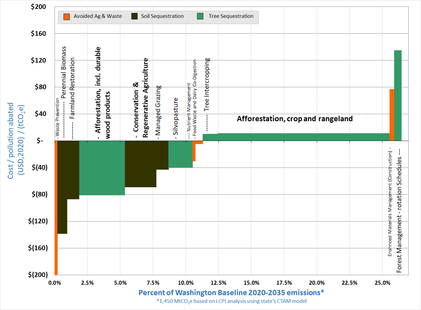
Figure 5 – Washington 2020-2035 MAC for Agriculture, Forestry, & Waste measures.
% of Washington Baseline 2020-2035 emissions: 26.5% (380 MtCO2e)
Average Abatement Cost of all options: -$27/tCO2e (-$976 to $135)
Sources of information and methodology notes: Measures incorporated are from Project Drawdown Plausible Scenario and the Oregon MAC Curve study Scenario 1 or Scenario 2 (afforestation only).
Project Drawdown generally assumes linear adoption rates for measures from 2020-2050. Those are scaled back to 2020-2035 for this analysis. Project Drawdown solutions identified as relevant to Washington state were by typically scaled by share of global cropland or agricultural land (0.3%).
Oregon values are for 2022-2035, cost adjusted from the original study (USD, 2010) to USD, 2020. The Oregon study reported cumulative values through 2022 and 2035 respectively, the difference of the two was used to project impacts from 2022-2035, roughly consistent with the 2020-2035 window used throughout this CaPI analysis. Afforestation is scaled by relative cropland and rangeland acreage in Washington versus Oregon. Other measures are either do not have scaling applied or are scaled by cropland acreage or population.
See the Appendix for more measure-specific details.
Other Sectors
Figure 6 presents a “zoomed-in” look at some Transport, Residential/Commercial/Industrial Fuel Switch, and Power Generation measures applicable to Washington state. A short summary of each sector is provided below, and more detail is provided for each measure in the Appendix.
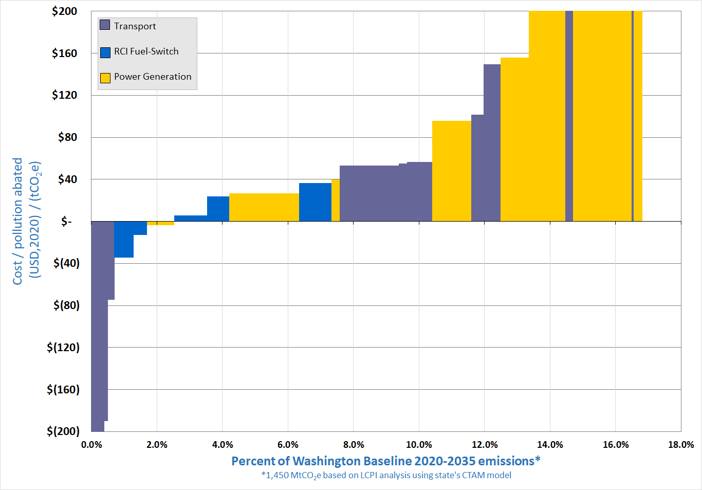
Figure 6 – Washington 2020-2035 MAC for Transportation, RCI Fuel Switch, and Power Generation measures.
% of Washington Baseline 2020-2035 emissions: 8.4% (120 MtCO2e) 1Average Abatement Cost of all options: $214/tCO2e (-$3.5 to $1,162)
Main Sources of Information:
- E3 PGP Study
- NPCC 7th Northwest Power Plan
- Oregon MAC Curve
- Department of Commerce Carbon Tax Assessment Model (CTAM)
- Department of Commerce Fuel Mix Disclosure Reports
- EIA State Energy Data System
Transportation
% of Washington Baseline 2020-2035 emissions: 4.7% (MtCO2e)
Average Abatement Cost of all options: $70/tCO2e (-$1,028 to $1,010)
Main Sources of Information:
Residential, Commercial, Industrial Fuel Switch
% of Washington Baseline 2020-2035 emissions: 3.7% (50 MtCO2e)2Average Abatement Cost of all options: $9/tCO2e (-$35 to $37)
Main Sources of Information:
Appendix: Table of all Measures

